Exponential & logistic growth
Exponential & logistic growth
Modeling population growth rates
To understand the different models that are used to represent population dynamics, let's start by looking at a general equation for the population growth rate (change in number of individuals in a population over time):

In this equation, dN/dT is the growth rate of the population a given instant, N is population size, T is time, and r is the per capita rate of increase –that is, how quickly the population grows per individual already in the population.
If we assume no movement of individuals into or out of the population, r is just a function of birth and death rates. You can learn more about the meaning and derivation of the equation here:
The equation above is very general, and we can make more specific forms of it to describe two different kinds of growth models: exponential and logistic.
- When the per capita rate of increase (r) takes the same positive value regardless of the population size, then we get exponential growth.
- When the per capita rate of increase (r) decreases as the population increases towards a maximum limit, then we get logistic growth.

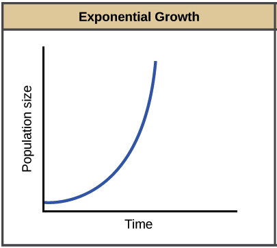
Exponential growth
Bacteria grown in the lab provide an excellent example of exponential growth. In exponential growth, the population’s growth rate increases over time, in proportion to the size of the population.
Let’s take a look at how this works. Bacteria reproduce by binary fission (splitting in half), and the time between divisions is about an hour for many bacterial species. To see how this exponential growth, let's start by placing bacteria in a flask with an unlimited supply of nutrients.
- After hour: Each bacterium will divide, yielding bacteria (an increase of bacteria).
- After hours: Each of the bacteria will divide, producing (an increase of bacteria).
- After hours: Each of the bacteria will divide, producing (an increase of bacteria).
The key concept of exponential growth is that the population growth rate —the number of organisms added in each generation—increases as the population gets larger. And the results can be dramatic: after day ( cycles of division), our bacterial population would have grown from to over billion! When population size, , is plotted over time, a J-shaped growth curve is made.
How do we model the exponential growth of a population? As we mentioned briefly above, we get exponential growth when (the per capita rate of increase) for our population is positive and constant. While any positive, constant can lead to exponential growth, you will often see exponential growth represented with an of .
is the maximum per capita rate of increase for a particular species under ideal conditions, and it varies from species to species. For instance, bacteria can reproduce much faster than humans, and would have a higher maximum per capita rate of increase. The maximum population growth rate for a species, sometimes called its biotic potential, is expressed in the following equation:

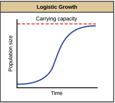
Logistic growth
Exponential growth is not a very sustainable state of affairs, since it depends on infinite amounts of resources (which tend not to exist in the real world).
Exponential growth may happen for a while, if there are few individuals and many resources. But when the number of individuals gets large enough, resources start to get used up, slowing the growth rate. Eventually, the growth rate will plateau, or level off, making an S-shaped curve. The population size at which it levels off, which represents the maximum population size a particular environment can support, is called the carrying capacity, or K.
We can mathematically model logistic growth by modifying our equation for exponential growth, using an r (per capita growth rate) that depends on population size (N) and how close it is to carrying capacity (K). Assuming that the population has a base growth rate of r max when it is very small, we can write the following equation:
Let's take a minute to dissect this equation and see why it makes sense. At any given point in time during a population's growth, the expression K-N tells us how many more individuals can be added to the population before it hits carrying capacity. (K - N)/K, then, is the fraction of the carrying capacity that has not yet been “used up.” The more carrying capacity that has been used up, the more the (K - N)/K term will reduce the growth rate.
When the population is tiny, N is very small compared to K. The (K - N)/K term becomes approximately (K/K) or 1, giving us back the exponential equation. This fits with our graph above: the population grows near-exponentially at first, but levels off more and more as it approaches K
Role of intraspecific competition
The logistic model assumes that every individual within a population will have equal access to resources and, thus, an equal chance for survival. For plants, the amount of water, sunlight, nutrients, and the space to grow are the important resources, whereas in animals, important resources include food, water, shelter, nesting space, and mates.
In the real world, the variation of phenotypes among individuals within a population means that some individuals will be better adapted to their environment than others. The resulting competition between population members of the same species for resources is termed intraspecific competition (intra- = "within"; -specific = "species"). Intraspecific competition for resources may not affect populations that are well below their carrying capacity as resources are plentiful and all individuals can obtain what they need. However, as population size increases, this competition intensifies. In addition, the accumulation of waste products can reduce an environment's carrying capacity.
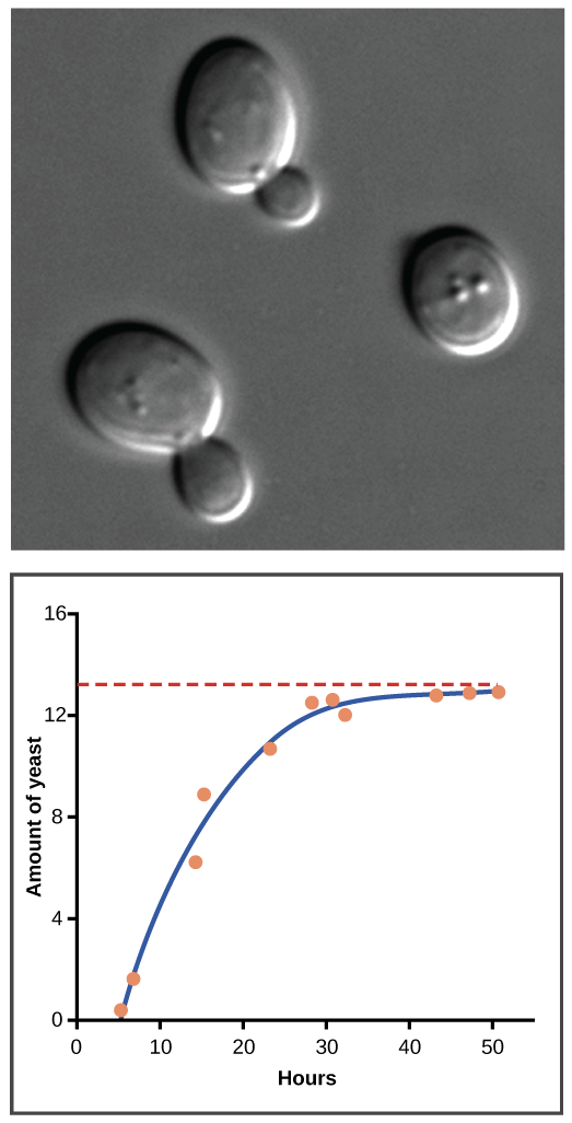
Examples of logistic growthYeast, a microscopic fungus used to make bread and alcoholic beverages, can produce a classic S-shaped curve when grown in a test tube. In the graph shown below, yeast growth levels off as the population hits the limit of the available nutrients. (If we followed the population for longer, it would likely crash, since the test tube is a closed system – meaning that fuel sources would eventually run out and wastes might reach toxic levels).
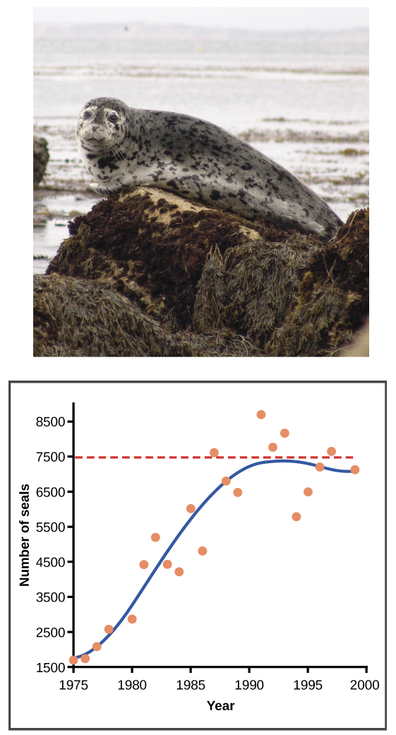
In the real world, there are variations on the “ideal” logistic curve. We can see one example in the graph below, which illustrates population growth in harbor seals in Washington State. In the early part of the 20th century, seals were actively hunted under a government program that viewed them as harmful predators, greatly reducing their numbers. Since this program was shut down, seal populations have rebounded in a roughly logistic pattern


woww informasinya sangat jelas dan rapi. tapi dapatkah individu yang termasuk exponential growth menjadi logistic growth dan sebaliknya? terimakasih :)
BalasHapus